Line Drawing Algorithms and a Neural Approximation
I was studying line drawing algorithms and then had an idea to replace the best algorithm with a neural network. This long post contains an explanation of the basic algorithms and the process I went through to mimick the best algorithm.
So I coded up three line drawing algorithms that I read on Wikipedia. Let's start from the most basic one.
Naive Algorithm
std::vector<std::vector<int>> naive(float x1, float y1, float x2, float y2) {
	assert(0 <= x1 and x1 < ZWIDTH);
	assert(0 <= x2 and x2 < ZWIDTH);
	assert(0 <= y1 and y1 < ZHEIGHT);
	assert(0 <= y2 and y2 < ZHEIGHT);

	if (x1 > x2) {
		std::swap(x1, x2);
		std::swap(y1, y2);
	}

	float dx = x2 - x1;
	float dy = y2 - y1;

	std::vector<std::vector<int>> image(HEIGHT, std::vector<int>(WIDTH));
	for (float x = x1, y; x <= x2; x++) {
		y = y1 + dy * (x - x1) / dx;
		int xx = static_cast<int>(x);
		int yy = static_cast<int>(y);
		color_square(image, xx, yy, 255);
	}

	return image;
}
We iterate over the $x$ coordinate and calculate the $y$ using the gradient. We round down the point to it's pixel and fill the pixel with white.
Unfortunately, this algorithm does not work well in all the cases. Often it leaves gaps in the lines depending upon whether the slope is greater than 1 or not in magnitude.
DDA Algorithm
This algorithm improves on the previous algorithm but accounting for all the cases.
std::vector<std::vector<int>> dda(float x1, float y1, float x2, float y2) {
	if (x1 > x2) {
		std::swap(x1, x2);
		std::swap(y1, y2);
	}

	float dx = x2 - x1;
	float dy = y2 - y1;
	float step = std::max(fabs(dx), fabs(dy));
	dx /= step;
	dy /= step;

	std::vector<std::vector<int>> image(HEIGHT, std::vector<int>(WIDTH));
	for (float i = 0; i < step; i++) {
		int x = static_cast<int>(x1 + dx * i);
		int y = static_cast<int>(y1 + dy * i);
		color_square(image, x, y, 255);
	}

	return image;
}
We iterate over the larger of $\triangle X$ and $\triangle Y$ and calculate the $x$ and $y$ coorinates on the fly using gradient. We round down the point to it's pixel and fill the pixel.
Although, we get a connected line, the line appears jagged in a lot of cases.
Xiaolin Wu's Line Algorithm
The lines drawn by the previous two algorithms are not smooth. They are jagged. If we zoom out or see the image from a distance, the line won't appear smooth at all.
When two pixels of the image diagonal to each other are bright, then the pixel sharing edges with these two bright pixels should be slightly bright too for the smoothness. This is called anti-aliasing. The question now becomes that which pixels should be given brightness and how much brightness should they be given. This calcualtion problem is solved by this algorithm.
The following is the code for it. The pseudocode has been given on Wikipedia. I merely converted it to C++.
std::vector<std::vector<int>> wu(float x1, float y1, float x2, float y2) {
	bool steep = std::abs(y2 - y1) > std::abs(x2 - x1);
	if (steep) {
		std::swap(x1, y1);
		std::swap(x2, y2);
	}
	if (x1 > x2) {
		std::swap(x1, x2);
		std::swap(y1, y2);
	}

	float dx = x2 - x1;
	float dy = y2 - y1;
	float gradient = dy / dx;
	if (dx == 0.0) gradient = 1.0;
	std::vector<std::vector<int>> image(HEIGHT, std::vector<int>(WIDTH));

	float xend;
	float yend;
	float xgap;

	// handle first endpoint
	xend = std::round(x1);
	yend = y1 + gradient * (xend - x1);
	xgap = rfpart(x1 + 0.5);
	float xpxl1 = xend;
	float ypxl1 = std::floor(yend);

	if (steep) {
		color_square(image, ypxl1, xpxl1, static_cast<int>((rfpart(yend) * xgap) * 255));
		color_square(image, ypxl1 + 1, xpxl1, static_cast<int>((fpart(yend) * xgap) * 255));
	} else {
		color_square(image, xpxl1, ypxl1, static_cast<int>((rfpart(yend) * xgap) * 255));
		color_square(image, xpxl1 + 1, ypxl1, static_cast<int>((fpart(yend) * xgap) * 255));
	}
	float intery = yend + gradient;

	// handle second endpoint
	xend = std::round(x2);
	yend = y2 + gradient * (xend - x2);
	xgap = rfpart(x2 + 0.5);
	float xpxl2 = xend;
	float ypxl2 = std::floor(yend);

	if (steep) {
		color_square(image, ypxl2, xpxl2, static_cast<int>((rfpart(yend) * xgap) * 255));
		color_square(image, ypxl2 + 1, xpxl2, static_cast<int>((fpart(yend) * xgap) * 255));
	} else {
		color_square(image, xpxl2, ypxl2, static_cast<int>((rfpart(yend) * xgap) * 255));
		color_square(image, xpxl2 + 1, ypxl2, static_cast<int>((fpart(yend) * xgap) * 255));
	}

	if (steep) {
		for (float x = xpxl1 + 1; x < xpxl2; x += 1) {
			color_square(image, std::floor(intery), x, static_cast<int>((rfpart(intery)) * 255));
			color_square(image, std::floor(intery) + 1, x, static_cast<int>((fpart(intery)) * 255));
			intery = intery + gradient;
		}
	} else {
		for (float x = xpxl1 + 1; x < xpxl2; x += 1) {
			color_square(image, x, std::floor(intery), static_cast<int>((rfpart(intery)) * 255));
			color_square(image, x, std::floor(intery) + 1, static_cast<int>((fpart(intery)) * 255));
			intery = intery + gradient;
		}
	}

	return image;
}
Let us not worry about the case when the line is steep as of now (steep means $\mid \frac{\triangle Y}{\triangle X} \mid \gt 1$).
Assuming $\mid \frac{\triangle Y}{\triangle X} \mid \le 1$, we walk more along the X-axis and less along the Y-axis for our line drawing algorithm. This means that if in our loop we iterate over the values of X, then we can gain finer control over the drawing process since the resolution in X-direction is more.
We first draw the two endpoints beforehand and then using the algorithm fill the gaps between the two points.
We initiate our $x$ and $y$ to the smaller of the two points (comparison by $X$) and then increment $x$ one by one in a loop till the value reaches the other endpoint. For each iteration we increment the $y$ value by $\frac{\triangle Y}{\triangle X}$ which accounts for one unit of increase in $x$.
The value $y$ is a fraction and the exact point $y$ lies somewhere in a pixel. Let $f = y - \lfloor y \rfloor$ and $rf = 1 - f$ i.e. they are the fractional and the remaining fractional part of $y$. We assign the pixel $(x, \lfloor y \rfloor)$ brightness corresponding to $rf$ and the pixel just below it $(x, \lfloor y \rfloor + 1)$ brightness corresponding to $f$. Here, 1 means fully white and 0 means fully black.
Let's look at why this assignment makes sense. The actual value $y$ lies somewhere between $\lfloor y \rfloor$ and $\lfloor y \rfloor + 1$ i.e. it lies somewhere in the pixel belonging to $(x, \lfloor y \rfloor)$. This means that part of the line corresponding to $rf$ size lies in the pixel and does it should get brightness corresponding to that value.
For example, assume $y = 4.25$. The pixel $(2, 4)$ actually holds all the values of $y$ from $y \in [4, 5)$. Since, our algorithm gave us the point $y = 4.25$ after adding the gradient, the region of the line from $4.25$ to $4.9999999$ belongs to the pixel. Thus $rf$ should be the brightness value.
Now, the case for the steep slope is similar to in every way to the discussed case. It's just that we iterate over $y$ for higher resolution and we add the inverse of the gradient.
Comparison of the three algorithms
Image generated by the naive algorithm.
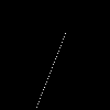
Image generated by the DDA algorithm.

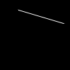
Image generated by Xiaolin Wu's DDA algorithm.
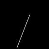
Open the images and zoom on them to see the differences.
Neural Network Line Drawing
I wanted to know whether we can replace the entire Xiaolin Wu's Algorithm with a neural network because why not.
Data Generation
Initially, I planned the Neural Network directly to output the image when I
give line coordinates so I generated images by applying Xiaolin Wu's Algorithm
on randomly chosen points on a 2 dimensional plane with each coordinate in the
range $(0, 100)$. I generated 1000 such images to train on in ppm format since
it is easiest to deal with this format programmatically. The format though is a
highly inefficient one since it stores the values for each pixel directly. I
then used the linux convert tool by ImageMagick to convert them into png
which reduced the size of the dataset by a lot by compression since most pixel
values were just black.
The code for image generation is below. The function wu is covered later and
the function write_image just writes the ppm image. I chose size 100 x 100
for the image so that the neural network does not get too big.
The input data is read from the coordinates.txt file for the neural network.
int main () {
	std::random_device rd;
	std::mt19937 mt(rd());
	std::uniform_real_distribution<float> dist(1.0f, static_cast<float>(WIDTH - 1));

	std::string rfname = "coordinates.txt";
	std::ofstream recordfile;
	recordfile.open(rfname);

	for (int i = 0; i < 1000; i++) {
		float x1 = dist(mt);
		float x2 = dist(mt);
		float y1 = dist(mt);
		float y2 = dist(mt);
		recordfile << x1 << " " << y1 << " " << x2 << " " << y2 << std::endl;
		auto image = wu(x1, y1, x2, y2);
		write_image(std::to_string(i) + ".ppm", image);
	}
	return 0;
}
Strategy 1 - Fully Connected Network with every pixel as an output.
I took a fully connected neural network and with 4 inputs and 10000 outputs. The inputs correspond to the x and y coordinates of two points in range (0, 100) which define the endpoints of the line. The outputs correspond to the pixels of a 100 x 100 square image. I tried out different number of layers - the minimum being 4 and the maximum being 12. I tried different sizes for these layers. I tried gradual increase in sizes and bottleneck architecture.
I trained the network for 5 epochs on the 1000 images that I generated. The error was not decreasing.
The best result I obtained with the lowest validation error is given below. The left image is the graph plotted by Wu's Algorithm for a given pair of points and the right image is the neural network's output image for the same set of points.
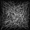
Nothing like a straight line, I know. But it is somewhat beautiful.
Strategy 2 - Fully Connected Network transitioning into a DeConvolutional Network
I had to read up on deconvolutional nerural networks and their architecture since I wanted to expand the output size with progression of layers.
So I took a deep FCN of about 5-6 layers, rolled up the output into a 2-D kernel and added a series of deconvolutional layers or transposed convolutional layers to increment the size of the image.
I tried different channel sizes and different layers in both the FCN and the DCNN. But the results always remained as follows for every input.
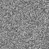
Sheer noise.
Strategy 3 - Try adding Positional Encoding
So while reading the NeRF series of papers I came across this concept of encoding the inputs in a different format to take them to a higher dimension to help learning of high frequency functions since Neural Networks are not so good at learning high frequency functions.
Every image is basically a signal (like sound). And the image signal is called high frequency when they gradient of the image is high. The gradient of the image is the difference between the adjacent pixels. So if the image is changing its pixel colours suddenly, then it is high frequency and neural networks are not good at approximating high freuqency functions with lower dimensional input.
So we take the input value $x$ and encode it into the different values $\sin(2^0 \pi x), \sin(2^1 \pi x), \sin(2^2 \pi x) \dots$ and so on. The idea is that some linear combination of these sine functions can approximate a higher order function and thus take our input to a higher dimension which can help the neural network to quickly approximate a high frequency function which would otherwise require several layers.
So I added this input encoding to the first two methods but sadly the result did not change at all. I think there was been a change but it was too feeble to notice.
Strategy 4 - Neural Network with Pixel Coordinates as input and Brightness as output + Positional Encoding
These ideas were not working and were too complex. For a simple thing such as drawing a line, the network must be also be simple. So I went with a slightly different approach.
Now the neural network is such that it takes, the 2 points as input which define the line to be drawn. It also takes $(i, j)$, the pixel coordinates as the input. The output of the network is a single value supposedly in the range $[0, 255]$ which defines the brightness of the pixel.
I trained this on my original dataset of the images that I created. The error was quite small and I thought that this would work out.
But unfortunately, during testing the resultant image formed by querying this neural network for each pixel in a 100 x 100 image was completely black. A complete black image will always have a very small error sine the line drawn takes up very small fraction of pixels. After training for multiple epochs too, the function was not converging to give a lower error.
After much thinking I realised that for this particular architecture of neural network the dataset was heavily skewed. The ratio of black pixels to white pixels more than $1000 : 1$.
So I needed to come up with a datset which had comparable amount of black pixels and non-black pixels. Extracting this from the existing data would have been time consuming and heavily inefficient so I decided to remake the dataset which I cover in the next section.
I kept the ratio of black pixels to non-black pixels exactly $2 : 1$.
The results were the best obtained so far. The left images are the images from Wu's Algorihm. The images on the right are from the Neural Network Queries. Both of them have the same input.
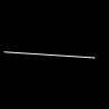
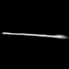
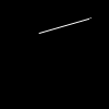
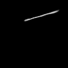
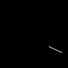
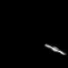
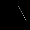
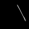
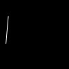
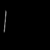
So I finally added positional encoding to check if any change occurs.
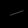
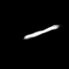
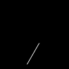
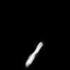
The lines got much thicker. And for smaller lines the output did not look like a line. So the model without positional encoding performed better.
New Dataset Generation
Rather than using the existing dataset in an inefficient manner, I remade the dataset according to the new requirement.
For each randomly generated pair of points, I took all the non-black pixels that come in the image in the dataset. And I also took twice this number of random black pixels for the same coordinate pair. This mean that the ratio of black to non-black pixels in the dataset is $2 : 1$ which is comparable to each other.
The code for the generation of the data is given below.
std::vector<std::array<float, 7>> differentdata(std::vector<std::vector<int>> &image, float x1, float x2, float y1, float y2) {
	std::vector<std::array<float, 7>> output;
	for (int i = 0; i < HEIGHT; i++) {
		for (int j = 0; j < WIDTH; j++) {
			if (image[i][j] != 0) {
				output.push_back({x1, y1, x2, y2,
						static_cast<float>(i), static_cast<float>(j), static_cast<float>(image[i][j])});
			}
		}
	}

	int not_black = output.size();
	while (output.size() < 3 * not_black) {
		int i = rand() % HEIGHT;
		int j = rand() % WIDTH;
		if (image[i][j] == 0) {
			output.push_back({x1, y1, x2, y2,
					static_cast<float>(i), static_cast<float>(j), static_cast<float>(image[i][j])});
		}
	}

	return output;
}

int main () {
	std::random_device rd;
	std::mt19937 mt(rd());
	std::uniform_real_distribution<float> dist(1.0f, static_cast<float>(WIDTH - 1));

	std::string rfname = "data.txt";
	std::ofstream recordfile;
	recordfile.open(rfname);
	recordfile << std::fixed << std::setprecision(6);

	for (int i = 0; i < 10000; i++) {
		float x1 = dist(mt);
		float x2 = dist(mt);
		float y1 = dist(mt);
		float y2 = dist(mt);
		auto image = wu(x1, y1, x2, y2);
		auto to_write = differentdata(image, x1, x2, y1, y2);
		for (auto oo : to_write) {
			for (float val : oo) recordfile << val << " ";
			recordfile << std::endl;
		}
	}
	return 0;
}
The pixel data is kept in a single file in which each row contains 7 values:
- 4 values to describe the endpoints
- 2 values to describe the pixel coordinate
- 1 value to describe the brightness of the pixel